
Overview – Inferential statistics
Inferential statistics are a way for researchers to work out whether findings from the particular sample they studied validly apply to the wider population. In other words, it’s a way for researchers to assess whether patterns or differences found in their data are likely to reflect an actual real-world effect rather than occurring by chance.
This page covers the key concepts needed to use inferential statistics in psychology:
- Probability – how likely it is that a result could occur by chance.
- Significance levels – using a probability value to decide whether a result is statistically significant (including type 1 and type 2 errors).
- Normal and skewed distributions – understanding the shape of data distributions and why this matters when selecting a statistical test.
- Parametric tests – statistical tests used when data meets specific criteria.
- Non-parametric tests – statistical tests that make fewer assumptions about the data (including how to calculate Chi-square for OCR and how to calculate the sign test for AQA).
Probability
Probability is a way of describing how likely something is to happen. In the context of psychological research, probability is used to work out how likely it is that a result could have happened by chance as opposed to the factor being studied.
For example, let’s say you are studying whether listening to music while studying improves memory. You give 100 students a memory test after they have studied a list of words, with half listening to music and half studying in silence. The students who listened to music remember an average of 22 words whereas those who studied in silence remember an average of 20 words. You might take these results to mean that listening to music improves memory. However, a difference of two words could have happened simply due to chance. So probability allows us to work out how likely it is that a difference this large could have occurred by chance rather than because listening to music genuinely affects memory.
A statistical test tells us how likely it is that the difference or relationship we found in our results could have happened by chance. This probability is usually expressed as a p-value (p). The smaller the p value, the less likely it is that the results occurred by chance. For example:
- p = 0.20 means there is a 20% probability of obtaining a result at least this extreme by chance, assuming there is no real effect.
- p = 0.03 means there is a 3% probability of obtaining a result at least this extreme by chance, assuming there is no real effect.
Researchers can then use this probability to decide whether a finding is statistically significant (see below).
Significance levels
A significance level is the probability that researchers set to decide whether a result counts as statistically significant (or not).
In psychology, researchers commonly use a significance threshold of p < 0.05. This means that there would be less than a 5% chance of obtaining this result purely by luck if there were no real effect.
So, we work out the p-value (p) of our results. Assuming a significance threshold of p < 0.05:
- If p = 0.03, we would say the results are statistically significant because 0.03 < 0.05
- If p = 0.20, we would say the results are not statistically significant because 0.20 > 0.05
If a result is statistically significant, researchers reject the null hypothesis and conclude that there is sufficient evidence of a difference or relationship.
If the result is not statistically significant, researchers fail to reject the null hypothesis. However, this does not prove that there is no effect – it just means that the evidence is not strong enough to conclude that there is a statistically significant effect.
Type 1 and type 2 errors
Statistical decisions are not always correct. Researchers can make two kinds of errors:
- Type 1 error (false positive): The researcher concludes that there is a significant effect when there is actually no real effect. In other words, they reject the null hypothesis when it is actually true.
- E.g. the researchers set the p threshold as <0.05 but the researchers’ results are among the 5% of possible fluke outcomes that look significant but are just due to luck. So, they conclude there is an effect when there isn’t one in reality.
- Type 2 error (false negative): The researcher concludes that there is no significant effect when there is actually a real effect. In other words, they fail to reject the null hypothesis when it is actually false.
- There is a real effect and the researchers set the p threshold as <0.05. But their results are not among the 5% of possible results that would be considered statistically significant. So, they conclude there isn’t an effect when there actually is one in reality.
Basically, you can never rule out luck entirely no matter what the significance level and so it’s always possible the results suggest an effect when there isn’t one (type 1 error) or your results miss an effect that really exists (type 2 error).
Normal and skewed distributions
Before using some statistical tests, researchers need to consider how their data is distributed. Data can have a normal distribution or a skewed distribution.
Normal distribution
A normal distribution is when most scores are close to the mean with fewer and fewer scores the further you get from the mean.
A normal distribution is symmetrical like the diagram below. Scores are spread evenly on either side of the mean and create a bell-shaped curve where most scores create a peak in the middle that gets lower and lower the further you get from the mean.
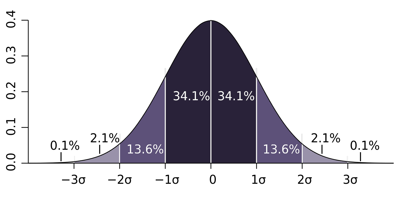
IQ scores are approximately normally distributed: most people have IQ scores close to the average, while very high and very low scores are less common.
Skewed distribution
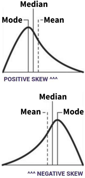 A skewed distribution is when the scores are not spread evenly around the mean. This can happen when there are outliers – unusually high or low scores that pull the mean towards them.
There are two types of skewed distribution:
- Positive skew: A few unusually high scores pull the mean upwards, so most scores are below the mean.
- Mean > median > mode
- Negative skew: A few unusually low scores pull the mean downwards, so most scores are above the mean.
- Mean < median < mode
The shape of the distribution is important because it helps determine which statistical test researchers should use:
- Parametric tests assume that the data is normally distributed.
- But if the data is strongly skewed, researchers may need to use a non-parametric statistical test.
Parametric tests
Parametric tests are used to test whether results are statistically significant. They are used when the data meets certain conditions:
- The data should be measured at interval (or ratio) level. For example, scores on an IQ test or reaction times in milliseconds.
- The data should be approximately normally distributed (i.e. the scores should form a roughly symmetrical, bell-shaped distribution rather than being strongly skewed).
- The data should be suitable for the particular test being used. For example, if you are comparing means scores you could use a t test, whereas if you are investigating correlations you could use Pearson’s r.
If these conditions are not met, researchers should use a non-parametric test instead.
Examples of parametric tests include:
- Related or unrelated t test: Used to test for a difference between two sets of interval data.
- Pearson’s r: Used to test for a correlation between two sets of interval data.
Non-parametric tests
Non-parametric tests are also used to test whether results are statistically significant. They are chosen when data does not meet the criteria for a parametric test – such as when the data has a skewed distribution or is in the ordinal or nominal format.
The choice of non-parametric test depends on the type of data, whether the groups are related or unrelated, and whether the researcher is testing for a difference or correlation:
- Mann-Whitney U: Used to test for a difference between two unrelated groups when the data is ordinal.
- For example, it could be used to compare the ranked anxiety scores of two different groups of participants.
- Wilcoxon Signed Ranks: Used to test for a difference between two related sets of scores when the data is ordinal.
- For example, it could be used to compare participants’ ranked anxiety scores before and after an intervention.
- Binomial Sign: Used to test for a difference between two related sets of scores when the data is nominal.
- For example, participants could be asked to choose between two options before and after an intervention, and the researcher could compare the frequencies of each response.
- Spearman’s Rho: Used to test for a correlation when the data is ordinal.
- For example, it could be used to investigate whether there is a relationship between ranked stress levels and ranked sleep quality.
- Chi-squared: Used with nominal data when the researcher is comparing frequencies.
- For example, it could be used to test whether participants in different experimental conditions are more likely to follow or disobey an instruction.
| Type | Test | When to use |
|---|---|---|
| Parametric (normally distributed data – not really relevant for A-level psychology) |
Unrelated t test | Two unrelated groups Interval data Normally distributed |
| Related t test | Two related sets of scores Interval data Normally distributed |
|
| Pearson’s r | Correlation Interval data Normally distributed |
|
| Non-parametric (skewed distribution or ordinal/nominal data) |
Mann-Whitney U | Two unrelated groups Ordinal data |
| Wilcoxon Signed Ranks | Two related sets of scores Ordinal data |
|
| Chi-squared | Nominal data Frequencies are being compared |
|
| Binomial Sign | Two related sets of scores Nominal data |
|
| Spearman’s Rho | Correlation Ordinal data |
How to calculate chi-squared
Note: The OCR spec lists being able to calculate chi-squared, whereas the AQA spec lists being able to calculate the sign test (below).
The chi-squared test is a way to calculate the statistical significance of a difference or relationship between nominal data. It is used when the data consists of frequencies – i.e. the number of people or observations in each category.
You basically need to work out two numbers:
- The chi-squared value
- The critical value
Your results are statistically significant if the chi-squared value is equal to or greater than the critical value.
Example: Let’s say we want to investigate whether participants in different experimental conditions are more likely to follow or disobey an instruction. We have 20 participants, with 10 in each condition.
| Follow | Disobey | Total | |
| Condition A | 8 | 2 | 10 |
| Condition B | 4 | 6 | 10 |
| Total | 12 | 8 | 20 |
- The first thing to do is record the observed frequencies (O). These are the actual results collected by the researchers (see the table above).
- Condition A + Follow = 8
- Condition A + Disobey = 2
- Condition B + Follow = 4
- Condition B + Disobey = 6
- Next, work out the expected frequencies (E). These are the frequencies we would expect to get if there were no relationship between the experimental condition and whether participants followed or disobeyed the instruction.
- The expected frequency is calculated using:
- E = (row total × column total) ÷ overall total
- So, in this example, the expected frequencies are:
- Condition A + Follow = ((10 × 12) ÷ 20) = 6
- Condition A + Disobey = ((10 × 8) ÷ 20) = 4
- Condition B + Follow = ((10 × 12) ÷ 20) = 6
- Condition B + Disobey = ((10 × 8) ÷ 20) = 4
- The expected frequency is calculated using:
- We can then use these observed and expected frequencies to calculate the chi-squared value (χ²)
- For each category, work out the difference between the observed and expected frequency, e.g.:
- Condition A + Follow = (8 – 6) = 2
- Condition A + Disobey = (2 – 4) = -2
- Condition B + Follow = (4 – 6) = -2
- Condition B + Disobey = (6 – 4) = 2
- Square each difference and divide it by the expected frequency, e.g.:
- Condition A + Follow = (2² ÷ 6) = 0.67
- Condition A + Disobey = (-2² ÷ 4) = 1
- Condition B + Follow = (-2² ÷ 6) = 0.67
- Condition B + Disobey = (2² ÷ 4) = 1
- Add the results for all categories together.
- E.g. 0.67 + 1 + 0.67 + 1 = 3.33
- So for this example:
- χ² = 3.33
- For each category, work out the difference between the observed and expected frequency, e.g.:
- Next, work out the critical value:
- Calculate the degrees of freedom (df):
- df = (number of rows − 1) × (number of columns − 1)
- There are 2 rows and 2 columns, so:
- df = (2 − 1) × (2 − 1) = 1
- Find out the p value required for the test (this will be provided in the exam)
- For example, let’s say we are using p = 0.05.
- Using the degrees of freedom and p value, look up the critical value (cv) in a chi-squared critical values table (this will be provided in the exam)
- So, in this example:
- df = 1
- p = 0.05
- So our critical value (cv) is 3.84.
- So, in this example:
- Calculate the degrees of freedom (df):
- Compare the calculated chi-squared value with the critical value
- In this example, our chi-squared value (χ²) value is 3.33, which is below out critical value of 3.84.
- Because 3.33 is less than 3.84, the result is not statistically significant
- This means we accept the null hypothesis and reject the experimental hypothesis.
How to calculate sign test
Note: The AQA spec lists being able to the sign test, whereas the OCR spec lists being able to calculate chi-squared (above).
The sign test is a way to calculate the statistical significance of differences between related pairs (e.g. before and after in a repeated measures experiment) of nominal data.
You basically need to work out two numbers:
- The observed value
- The critical value
If the observed value (s) is equal or less than the critical value (cv), the results are statistically significant.
Example: Let’s say we ran an experiment on 10 participants to see whether they prefer movie A or movie B.
| Participant | Movie A rating |
Movie B rating |
Sign |
| A | 3 | 6 | B |
| B | 3 | 3 | n/a |
| C | 5 | 6 | B |
| D | 4 | 6 | B |
| E | 2 | 3 | B |
| F | 3 | 7 | B |
| G | 5 | 3 | A |
| H | 7 | 8 | B |
| I | 2 | 6 | B |
| J | 8 | 5 | A |
- The most important thing in the sign test is not the actual amount (e.g. 4, 6, etc.), but the sign – i.e. whether they preferred movie A or movie B. You exclude any results that are the same between the pairs.
- n = 9 (because even though there are 10 participants, one participant had no change so we exclude them from our calculation)
- B = 7
- A = 2
- Look to see if your experimental hypothesis is two-tailed (i.e. a change is expected in either direction) or one-tailed (i.e. change is expected to go in one direction)
- In this case our experimental hypothesis is two-tailed: Participants may prefer movie A or movie B
- (The null hypothesis is that participants like both movies equally)
- Find out the p value for the example (this will be provided in the exam)
- In this case, let’s say it’s 0.1
- Using the information above, look up your critical value (cv) in a critical values table (this will be provided in the exam)
- In this example:
- n = 9
- p = 0.1
- The experimental hypothesis is two-tailed
- So our critical value (cv) is 1
- In this example:
- Work out the observed value (s) by counting the number of instances of the less frequently occurring sign (A in this case)
- In this example, there are 2 As, so our observed value (s) is 2
- Compare the observed value with the critical value
- In this example, the observed value (2) is greater than the critical value (1) and so the results are not statistically significant.
- This means we must accept the null hypothesis and reject the experimental hypothesis.
- In this example, the observed value (2) is greater than the critical value (1) and so the results are not statistically significant.