Overview – Research Methods

Research methods are how psychologists and scientists come up with and test their theories. The A level psychology syllabus covers several different types of studies and experiments used in psychology as well as how these studies are conducted and reported:

• Types of psychological studies (including experiments, observations, self-reporting, and case studies)
• Scientific processes (including the features of a study, how findings are reported, and the features of science in general)
• Data handling and analysis (including descriptive statistics and different ways of presenting data) and inferential testing

Note: Unlike all other sections across the 3 exam papers, research methods is worth 48 marks instead of 24. Not only that, the other sections often include a few research methods questions, so this topic is the most important on the syllabus!

---

Practice papers with A* answers book #2 contains five full exam papers with five research methods sections. These questions cover the different types of study, how findings are reported, and have several worked examples of those tricky maths questions! 

Example question: Design a matched pairs experiment the researchers could conduct to investigate differences in toy preferences between boys and girls. [12 marks]

---

Types of study

---

There are several different ways a psychologist can research the mind, including:

• Experiments
• Observation
• Self-reporting
• Case studies

Each of these methods has its strengths and weaknesses. Different methods may be better suited to different research studies.

Experimental method

The experimental method looks at how variables affect outcomes. A variable is anything that changes between two situations (see below for the different types of variables). For example, Bandura’s Bobo the doll experiment looked at how changing the variable of the role model’s behaviour affected how the child played.

Experimental designs

Experiments can be designed in different ways, such as:

• Independent groups: Participants are divided into two groups. One group does the experiment with variable 1, the other group does the experiment with variable 2. Results are compared.
• Repeated measures: Participants are not divided into groups. Instead, all participants do the experiment with variable 1, then afterwards the same participants do the experiment with variable 2. Results are compared.

A matched pairs design is another form of independent groups design. Participants are selected. Then, the researchers recruit another group of participants one-by-one to match the characteristics of each member of the original group. This provides two groups that are relevantly similar and controls for differences between groups that might skew results. The experiment is then conducted as a normal independent groups design.

Types of experiment

Laboratory vs. field experiment

Experiments are carried out in two different types of settings:

• Laboratory experiment: An experiment conducted in an artificial, controlled environment
  • E.g. Bandura’s Bobo the doll experiment or Asch’s conformity experiments
• Field experiment: An experiment carried out in a natural, real-world environment
  • E.g. Bickman’s study of the effects of uniforms on obedience

Natural and quasi experiment

Natural experiments are where variables vary naturally. In other words, the researcher can’t or doesn’t manipulate the variables. There are two types of natural experiment:

• Natural experiment: An experiment where the variable changes naturally and the researcher seizes the opportunity to study the effects
  • E.g. studying the effect a change in drug laws (variable) has on addiction
• Quasi experiment: An experiment that compares between two variables that cannot be changed
  • E.g. studying differences between men (variable) and women (variable)

Observational method

The observational method looks at and examines behaviour. For example, Zimbardo’s prison study observed how participants behaved when given certain social roles.

Observational design

Behavioural categories

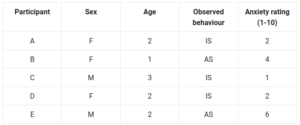
An observational study will use behavioural categories to prioritise which behaviours are recorded and ensure the different observers are consistent in what they are looking for.

For example, a study of the effects of age and sex on stranger anxiety in infants might use the following behavioural categories to organise observational data:

Participant	Sex	Age	Observed behaviour	Anxiety rating (1-10)
A	F	2	IS	2
B	F	1	AS	4
C	M	3	IS	1
D	F	2	IS	2
E	M	2	AS	6

Rather than writing complete descriptions of behaviours, the behaviours can be coded into categories. For example, IS = interacted with stranger, and AS = avoided stranger. Researchers can also create numerical ratings to categorise behaviour, like the anxiety rating example above.

Event and time sampling

Because behaviour is constant and varied, it may not be possible to record every single behaviour during the observation period. So, in addition to categorising behaviour, study designers will also decide when to record a behaviour:

• Event sampling: Counting how many times the participant behaves in a certain way.
• Time sampling: Recording participant behaviour at regular time intervals. For example, making notes of the participant’s behaviour after every 1 minute has passed.

Note: Don’t get event and time sampling confused with participant sampling, which is how researchers select participants to study from a population.

Types of observation

Naturalistic vs. controlled

Observations can be made in either a naturalistic or a controlled setting:

• Naturalistic: Observations made in a real-life setting
  • E.g. setting up cameras in an office or school to observe how people interact in those environments
• Controlled: Observations made in an artificial setting set up for the purposes of observation
  • E.g. Ainsworth’s strange situation or Zimbardo’s prison study

Covert vs. overt

Observations can be either covert or overt:

• Covert: Participants are not aware they are being observed as part of a study
  • E.g. setting up hidden cameras in an office
• Overt: Participants are aware they are being observed as part of a study
  • E.g. Zimbardo’s prison study

Participant vs. non-participant

In observational studies, the researcher/observer may or may not participate in the situation being observed:

• Participant observation: Where the researcher/observer is actively involved in the situation being observed
  • E.g. in Zimbardo’s prison study, Zimbardo played the role of prison superintendent himself
• Non-participant observation: When the researcher/observer is not involved in the situation being observed
  • E.g. in Bandura’s Bobo the doll experiment and Ainsworth’s strange situation, the observers did not interact with the children being observed

Self-report method

Self-report methods get participants to provide information about themselves. Information can be obtained via questionnaires or interviews.

Types of self-report

Questionnaires

A questionnaire is a standardised list of questions that all participants in a study answer. For example, Hazan and Shaver used questionnaires to collate self-reported data from participants in order to identify correlations between attachment as infants and romantic attachment as adults.

Questions in a questionnaire can be either open or closed:

• Closed questions: Have a fixed set of responses, such as yes/no or multiple choice questions.
  • E.g. “Are you religious?”
    • Yes
    • No
  • E.g. “How many hours do you spend online each day?”
    • <1 hour
    • 1-2 hours
    • 2-8 hours
    • >8 hours
• Open questions: Do not have a fixed set of responses, instead enabling participants to provide responses in their own words.
  • E.g. “How did you feel when you thought you were administering a lethal shock?” or “What do you look for in a romantic partner and why?”

Interviews

In an interview, participants are asked questions in person. For example, Bowlby interviewed 44 children when studying the effects of maternal deprivation.

Interviews can be either structured or unstructured:

• Structured interview: Questions are standardised and pre-set. The interviewer asks all participants the same questions in the same order.
• Unstructured interview: The interviewer discusses a topic with the participant in a less structured and more spontaneous way, pursuing avenues of discussion as they come up.

Interviews can also be a cross between the two – these are called semi-structured interviews.

Case studies

Note: This topic is A level only, you don’t need to learn about case studies if you are taking the AS exam only.

Case studies are detailed investigations into an individual, a group of people, or an event. For example, the biopsychology page describes a case study of a young boy who had the left hemisphere of his brain removed and the effects this had on his language skills.

In a case study, researchers use many of the methods described above – observation, questionnaires, interviews – to gather data on a subject. However, because case studies are studies of a single subject, the data they provide is primarily qualitative rather than quantitative. This data is then used to build a case history of the subject. Researchers then interpret this case history to draw their conclusions.

Types of case study

Typical vs. unusual cases

Most case studies focus on unusual individuals, groups, and events.

Longitudinal

Many case studies are longitudinal. This means they take place over an extended time period, with researchers checking in with the subject at various intervals. For example, the case study of the boy who had his left hemisphere removed collected data on the boy’s language skills at ages 2.5, 4, and 14 to see how he progressed.

---

Scientific processes

---

This section looks at how science works more generally – in particular how scientific studies are organised and reported. It also covers ways of evaluating a scientific study.

Study features and design

Aim

Studies will usually have an aim. The aim of a study is a description of what the researchers are investigating and why. For example, “to investigate the effect of SSRIs on symptoms of depression” or “to understand the effect uniforms have on obedience to authority”.

Hypothesis

Studies seek to test a hypothesis. The experimental/alternate hypothesis of a study is a testable prediction of what the researchers expect to happen.

• Experimental hypothesis: A prediction that changing the independent variable will cause a change in the dependent variable.
  • E.g. “That SSRIs will reduce symptoms of depression” or “subjects are more likely to comply when orders are issued by someone wearing a uniform”.
• Null hypothesis: A prediction that changing the independent variable will have no effect on the dependent variable.
  • E.g. “That SSRIs have no effect on symptoms on depression” or “subject conformity will be the same when orders are issued by someone wearing a uniform as when orders are issued by someone bot wearing a uniform”

Either the experimental/alternate hypothesis or the null hypothesis will be supported by the results of the experiment.

Sampling

It’s often not possible or practical to conduct research on everyone your study is supposed to apply to. So, researchers use sampling to select participants for their study.

• Population: The entire group that the study is supposed to apply to
  • E.g. all humans, all women, all men, all children, etc.
• Sample: A part of the population that is representative of the entire group
  • E.g. 10,000 humans, 200 women from the USA, children at a certain school

For example, the target population (i.e. who the results apply to) of Asch’s conformity experiments is all humans – but Asch didn’t conduct the experiment on that many people! Instead, Asch recruited 123 males and generalised the findings from this sample to the rest of the population.

Researchers choose from different sampling techniques – each has strengths and weaknesses.

Sampling techniques

Random sampling

The random sampling method involves selecting participants from a target population at random – such as by drawing names from a hat or using a computer program to select them. This method means each member of the population has an equal chance of being selected and thus is not subject to any bias.

Systematic sampling

The systematic sampling method involves selecting participants from a target population by selecting them at pre-set intervals. For example, selecting every 50th person from a list, or every 7th, or whatever the interval is.

Stratified sampling

The stratified sampling method involves dividing the population into relevant groups for study, working out what percentage of the population is in each group, and then randomly sampling the population according to these percentages.

For example, let’s say 20% of the population is aged 0-18, and 50% of the population is aged 19-65, and 30% of the population is aged >65. A stratified sample of 100 participants would randomly select 20x 0-18 year olds, 50x 19-65 year olds, and 30x people over 65.

Opportunity and volunteer sampling

The opportunity and volunteer sampling methods:

• Opportunity sampling: Approaching participants who are available and asking them to take part.
  • E.g. Approaching people in the street and asking them to complete a questionnaire.
• Volunteer sampling: Participants offer to take part (also called self-selected sampling).
  • E.g. Placing an advert online inviting people to complete a questionnaire.

Variables

Independent vs. dependent variables

If the study involves an experiment, the researchers will alter an independent variable to measure its effects on a dependent variable:

• Independent variable: Something that is changed by researchers in an experiment.
  • E.g. In Bickman’s study of the effects of uniforms on obedience, the independent variable was the uniform of the person giving orders.
• Dependent variable: Something that is measured by researchers in an experiment.
  • E.g. In Bickman’s study of the effects of uniforms on obedience, the dependent variable was how many people followed the orders.

Extraneous and confounding variables

In addition to the variables actually being investigated (independent and dependent), there may be additional (unwanted) variables in the experiment. These additional variables are called extraneous variables.

Researchers must control for extraneous variables to prevent them from skewing the results and leading to false conclusions. When extraneous variables are not properly controlled for they are known as confounding variables.

For example, if you’re studying the effect of caffeine on reaction times, it might make sense to conduct all experiments at the same time of day to prevent this extraneous variable from confounding the results. Reaction times change throughout the day and so if you test one group of subjects at 3pm and another group right before they go to bed, you may falsely conclude that the second group had slower reaction times.

Operationalisation of variables

Operationalisation of variables is where researchers clearly and measurably define the variables in their study.

For example, an experiment on the effects of sleep (independent variable) on anxiety (dependent variable) would need to clearly operationalise each variable. Sleep could be defined by number of hours spent in bed, but anxiety is a bit more abstract and so researchers would need to operationalise (i.e. define) anxiety such that it can be quantified in a measurable and objective way.

If variables are not properly operationalised, the experiment cannot be properly replicated, experimenters’ subjective interpretations may skew results, and the findings may not be valid.

Pilot studies

A pilot study is basically a practice run of the proposed research project. Researchers will use a small number of participants and run through the procedure with them. The purpose of this is to identify any problems or areas for improvement in the study design before conducting the research in full. A pilot study may also give an early indication of whether the results will be statistically significant.

For example, if a task is too easy for participants, or it’s too obvious what the real purpose of an experiment is, or questions in a questionnaire are ambiguous, then the results may not be valid. Conducting a pilot study first may save time and money as it enables researchers to identify and address such issues before conducting the full study on thousands of participants.

Study reporting

Features of a psychological report

The report of a psychological study (research paper) typically contains the following sections in the following order:

• Title: A short and clear description of the research.
• Abstract: A summary of the research. This typically includes the aim and hypothesis, methods, results, and conclusion.
• Introduction: Funnel technique: Broad overview of the context (e.g. current theories, previous studies, etc.) before focusing in on this particular study, why it was conducted, its aims and hypothesis.
• Method: A detailed description of the procedure used in the study, so that the study can be evaluated and replicated. Typically includes the following sub-sections (if appropriate):
  • Study design: This will explain what method was used (e.g. experiment or observation), how the study was designed (e.g. independent groups or repeated measures), and identification and operationalisation of variables.
  • Participants: A description of the target population to be studied, the sampling method, how many participants were included.
  • Equipment used: A description of any special equipment used in the study and how it was used.
  • Standardised procedure: A detailed step-by-step description of how the study was conducted. This allows for the study to be replicated by other researchers.
  • Controls: An explanation of how extraneous variables were controlled for so as to generate accurate results.
• Results: A presentation of the key findings from the data collected. This is typically written summaries of the raw data (descriptive statistics), which may also be presented in tables, charts, graphs, etc. The raw data itself is typically included in appendices.
• Discussion: An explanation of what the results mean and how they relate to the experimental hypothesis (supporting or contradicting it), any issues with how results were generated, how the results fit with other research, and suggestions for future research.
• Conclusion: A short summary of the key findings from the study.
• References: A list of all the sources – i.e. books and published articles – used in the study. These are listed according to standard formats, e.g. the Harvard referencing style:
  • Book: Milgram, S., 2010. Obedience to Authority. 1st ed. Pinter & Martin.
  • Journal article: Bandura, A., Ross, D. and Ross, S., 1961. Transmission of Aggression through Imitation of Aggressive Models. The Journal of Abnormal and Social Psychology, 63(3), pp.575-582.
• Appendices: This is where you put any supporting materials that are too detailed or long to include in the main report. For example, the raw data collected from a study, or the complete list of questions in a questionnaire.

Peer review

Peer review is a way of assessing the scientific credibility of a research paper before it is published in a scientific journal. The idea with peer review is to prevent false ideas and bad research from being accepted as fact.

It typically works as follows: The researchers submit their paper to the journal they want it to be published in, and the editor of that journal sends the paper to expert reviewers (i.e. psychologists who are experts in that area – the researchers’ ‘peers’) who evaluate the paper’s scientific validity. The reviewers may accept the paper as it is, accept it with a few changes, reject it and suggest revisions and resubmission at a later date, or reject it completely.

There are several different methods of peer review:

• Open review: The researchers and the reviewers are known to each other.
• Single-blind: The researchers do not know the names of the reviewers. This prevents the researchers from being able to influence the reviewer. This is the most common form of peer review.
• Double-blind: The researchers do not know the names of the reviewers, and the reviewers do not know the names of the researchers. This additionally prevents the reviewer’s bias towards the researcher from influencing their decision whether to accept their paper or not.

Study evaluation

Ethics

In psychological studies, ethical issues are questions of what is morally right and wrong. An ethically-conducted study will protect the health and safety of the participants involved and uphold their dignity, privacy, and rights.

To provide guidance on this, the British Psychological Association has published a code of human research ethics:

• Valid consent:
  • Participants are told the project’s aims, the data being collected, and any risks associated with participation.
  • Participants have the right to withdraw or modify their consent at any time.
  • Researchers can use incentives (e.g. money) to encourage participation, but these incentives can’t be so big that they would compromise a participant’s freedom of choice.
  • Researchers must consider the participant’s ability to consent (e.g. age, mental ability, etc.)
• No deception: Researchers should avoid misleading participants about the nature of the study wherever possible. However, some studies require a degree of deception (e.g. Asch’s conformity experiments wouldn’t have worked if participants were told the true nature of the test) and so in such cases the deception must be scientifically justified and researchers must use risk management to avoid harm. This may involve:
  • Prior (general) consent: Informing participants that they will be deceived without telling them the nature of the deception. However, this may affect their behaviour as they try to guess the real nature of the study.
  • Retrospective consent: Informing participants that they were deceived after the study is completed and asking for their consent. The problem with this is that if they don’t consent then it’s too late.
  • Presumptive consent: Asking people who aren’t participating in the study if they would be willing to participate in the study. If these people would be willing to give consent, then it may be reasonable to assume that those taking part in the study would also give consent.
• Confidentiality: Personal data obtained about participants should not be disclosed (unless the participant agreed to this in advance). Any data that is published will not be publicly identifiable as the participant’s.
• Debriefing: Once data gathering is complete, researchers must explain all relevant details of the study to participants – especially if deception was involved. If a study might have harmed the individual (e.g. its purpose was to induce a negative mood), it is ethical for the debrief to address this harm (e.g. by inducing a happy mood) so that the participant does not leave the study in a worse state than when they entered.

Reliability

Study results are reliable if the same results can be consistently replicated under the same circumstances. If results are inconsistent then the study is unreliable.

Note: Just because a study is reliable, its results are not automatically valid. A broken tape measure may reliably (i.e. consistently) record a person’s height as 200m, but that doesn’t mean this measurement is accurate.

There are several ways researchers can assess a study’s reliability:

Test-retest

Test-retest is when you give the same test to the same person on two different occasions. If the results are the same or similar both times, this suggests they are reliable.

For example, if your study used scales to measure participants’ weight, you would expect the scales to record the same (or a very similar) weight for the same person in the morning as in the evening. If the scales said the person weighed 100kg more later that same day, the scales (and therefore the results of the study) would be unreliable.

Inter-observer

Inter-observer reliability is a way to test the reliability of observational studies.

For example, if your study required observers to assess participants’ anxiety levels, you would expect different observers to grade the same behaviour in the same way. If one observer rated a participant’s behaviour a 3 for anxiety, and another observer rated the exact same behaviour an 8, the results would be unreliable.

Inter-observer reliability can be assessed mathematically by looking for correlation between observers’ scores. Inter-observer reliability can be improved by setting clearly defined behavioural categories.

Validity

Study results are valid if they accurately measure what they are supposed to. There are several ways researchers can assess a study’s validity:

• Concurrent validity: A test’s results are correlated with (i.e. similar to) the results of a similar test.
  • E.g. let’s say you come up with a new test to measure participants’ intelligence levels. If participants scoring highly on your test also scored highly on a standardised IQ test and vice versa, that would suggest your test has concurrent validity because participants’ scores are correlated with a known accurate test.
• Face validity: The study just looks like it measures what it’s supposed to at face value.
  • E.g. a study that measures participants’ intelligence levels by asking them when their birthday is would not have face validity. Getting participants to complete a standardised IQ test would have greater face validity.
• Ecological validity: The extent to which a study’s findings apply outside of the environment it was conducted in (i.e. in real life or other contexts).
  • E.g. let’s say your study was supposed to measure aggression levels in response to someone annoying. If the study was conducted in a lab and the participant knew they were taking part in a study, the results probably wouldn’t have much ecological validity because of the unrealistic environment.
• Temporal validity: The study’s results stay true over time.
  • E.g. a study conducted in 1920 that measured participants’ attitudes towards social issues may have low temporal validity because societal attitudes have changed since then.

Control of extraneous variables

There are several different types of extraneous variables that can reduce the validity of a study. A well-conducted psychological study will control for these extraneous variables so that they do not skew the results.

Demand characteristics

Demand characteristics are extraneous variables where the demands of a study make participants behave in ways they wouldn’t behave outside of the study. This reduces the study’s ecological validity.

For example, if a participant guesses the purpose of an experiment they are taking part in, they may try to please the researcher by behaving in the ‘right’ way rather than the way they would naturally. Alternatively, the participant might rebel against the study and deliberately try to sabotage it (e.g. by deliberately giving wrong answers).

In some study designs, researchers can control for demand characteristics using single-blind methods. For example, a drug trial could give half the participants the actual drug and the other half a placebo but not tell participants which treatment they received. This way, both groups will have equal demand characteristics and so any differences between them should be down to the drug itself.

Investigator effects

Investigator effects are another extraneous variable where the characteristics of the researcher affect the participant’s behaviour. Again, this reduces the study’s ecological validity.

Many characteristics – e.g. the researcher’s age, gender, accent, what they’re wearing – could potentially influence the participant’s responses. For example, in an interview about sex, females may feel less comfortable answering questions asked by a male interviewer and thus give different answers than if they were asked by a female. The researcher’s biases may also come across in their body language or tone of voice, affecting the participant’s responses.

In some study designs, researchers can control for demand characteristics using double-blind methods. In a double-blind drug trial, for example, neither the participants nor the researchers know which participants get the actual drug and which get the placebo. This way, the researcher is unable to give any clues (consciously or unconsciously) to participants that would affect their behaviour.

Participant variables

Participant variables are differences between participants. These can be controlled for by random allocation.

For example, in an experiment on the effect of caffeine on reaction times, participants would be randomly allocated into either the caffeine group or the non-caffeine group. A non-random allocation method, such as allocating caffeine to men and placebo to women, could mean variables in the allocation method (in this case gender) skew the results. When participants are randomly allocated, any extraneous variables (e.g. gender in this case) will be allocated evenly between each group and so not skew the results of one group more than the other.

Situational variables

Situational variables are the environment the experiment is conducted in. These can be controlled for by standardisation.

For example, all the tests of caffeine on reaction times would be conducted in the same room, at the same time of day, using the same equipment, and so on to prevent these features of the environment from skewing the results.

Task order

In a repeated measures experiment, researchers may use counterbalancing to control for the order in which tasks are completed.

For example, half of participants would do task A followed by task B, and the other half would do task B followed by task A.

Implications of psychological research for the economy

Psychological research often has practical applications in real life. The following are some examples of how psychological findings may affect the economy:

• Attachment: Bowlby’s maternal deprivation hypothesis suggests that periods of extended separation between mother and child before age 3 are harmful to the child’s psychological development. And if mothers stay at home during this period, they can’t go out to work. However, some more recent research challenges Bowlby’s conclusions, suggesting that substitutes (e.g. the father, or nursery care) can care for the child, allowing the mother to go back to work sooner and remain economically active.
• Psychopathology: Mental disorders affect people’s ability to work and so addressing these will likely have benefits for the economy. Further, psychologically healthy people are less likely to need use of health services or end up in prison, so psychological research may help save money in these areas. Examples:
  • Depression: Psychological research has found effective therapies for treating depression, such as cognitive behavioural therapy and SSRIs. The benefits of such therapies – if they are effective – are likely to outweigh the costs because they enable the person to return to work and pay taxes, as well avoiding long-term costs to the health service.
  • OCD: Similar to above: Drug therapies (e.g. SSRIs) and behavioural approaches (e.g. CBT) may alleviate OCD symptoms, enabling OCD sufferers to return to work, pay taxes, and avoid reliance on healthcare services.
• Memory: Public money is required to fund police investigations. Psychological tools, such as the cognitive interview, have improved the accuracy of eyewitness testimonies, which equates to more efficient use of police time and resources.

Features of science

Theory construction and hypothesis testing

Science works by making empirical observations of the world, formulating hypotheses/theories that explain these observations, and repeatedly testing these hypotheses/theories via experimentation.

Features of science

• Objectivity: Observations are made from a neutral perspective without bias, rather than the scientist’s subjective viewpoint.
  • E.g. A tape measure provides a more objective measurement of something compared to a researcher’s guess. Similarly, a set of scales is a more objective way of determining which of two objects is heavier than a researcher lifting each up and giving their opinion.
• Replicability: Scientific procedures and experiments can be repeated to double-check the findings are valid.
  • E.g. Burger (2009) replicated Milgram’s experiments with similar results.
• Falsifiability: When a theory or hypothesis is tested/replicated, there must be some possible observation that could prove it false – even if that never actually happens.
  • E.g. The hypothesis that “water boils at 100°c” could be falsified by an experiment where you heated water to 999°c and it didn’t boil. In contrast, “everything doubles in size every 10 seconds” could not be falsified by any experiment because whatever equipment you used to measure everything would also double in size.
  • Freud’s psychodynamic theories are often criticised for being unfalsifiable: There’s not really any observations that could disprove them because every possible behaviour (e.g. crying or not crying) could be explained as the result of some unconscious thought process.

Paradigm shifts

Philosopher Thomas Kuhn argues that science is not as unbiased and objective as it seems. Instead, the majority of scientists just accept the existing scientific theories (i.e. the existing paradigm) as true and then find data that supports these theories while ignoring/rejecting data that refutes them.

Rarely, though, minority voices are able to successfully challenge the existing paradigm and replace it with a new one. When this happens it is a paradigm shift. An example of a paradigm shift in science is that from Newtonian gravity to Einstein’s theory of general relativity.

---

Data handling and analysis

---

Types of data

Quantitative vs. qualitative

Data from studies can be quantitative or qualitative:

• Quantitative: Numerical
• Qualitative: Non-numerical

For example, some quantitative data in the Milgram experiment would be how many subjects delivered a lethal shock. In contrast, some qualitative data would be asking the subjects afterwards how they felt about delivering the lethal shock.

Content analysis

Although the detail of qualitative data may be valuable, this level of detail can also make it hard to objectively or mathematically analyse. Content analysis is a way of analysing qualitative data. The process is as follows:

• A sample of qualitative data is collected
  • E.g. A bunch of unstructured interviews on the topic of childhood
• Relevant coding units are identified and operationalised
  • E.g. Discussion of traumatic events, happy memories, births, and deaths
• The data is analysed according to these coding units to produce quantitative metrics
  • E.g. Researchers listen to the unstructured interviews and count how often traumatic events are mentioned
• Statistical analysis is carried out on this data

Primary vs. secondary

Researchers can produce primary data or use secondary data to achieve the research aims of their study:

• Primary data: Original data collected for the study
• Secondary data: Data from another study previously conducted

Meta-analysis

A meta-analysis is a study of studies. It involves taking several smaller studies within a certain research area and using statistics to identify similarities and trends within those studies to create a larger study.

We have looked at some examples of meta-analyses elsewhere in the course such as Van Ijzendoorn’s meta-analysis of several strange situation studies and Grootheest et al’s meta-analysis of twin studies on OCD.

A good meta-analysis is often more reliable than a regular study because it is based on a larger data set, and any issues with one single study will be balanced out by the other studies.

Descriptive statistics

Measures of central tendency: Mean, median, mode

Mean, median, and mode are measures of central tendency. In other words, they are ways of reducing large data sets into averages.

Mean

The mean is calculated by adding all the numbers in a set together and dividing the total by the number of numbers.

• Example set: 22, 78, 3, 33, 90
• 22+78+3+33+90=226
• 226/5=45.2
• The mean is 45.2

Median

The median is calculated by arranging all the numbers in a set from smallest to biggest and then finding the number in the middle. Note: If the total number of numbers is odd, you just pick the middle one. But if the total number of numbers is even, you take the mid-point between the two numbers in the middle.

• Example set: 20, 66, 85, 45, 18, 13, 90, 28, 9
• 9, 13, 18, 20, 28, 45, 66, 85, 90
• The median is 28

Mode

The mode is calculated by counting which is the most commonly occurring number in a set.

• Example set: 7, 7, 20, 16, 1, 20, 25, 16, 20, 9
• There are two 7’s, but three 20’s
• The mode is 20

Measures of dispersion: Range and standard deviation

Range and standard deviation are measures of dispersion. In other words, they quantify how much scores in a data set vary.

Range

The range is calculated by subtracting the smallest number in the data set from the largest number.

• Example set: 59, 8, 7, 84, 9, 49, 14, 75, 88, 11
• The largest number is 88
• The smallest number is 7
• 88-7=81
• The range is 81

Standard deviation

The standard deviation (σ) is a measure of how much numbers in a data set deviate from the mean (average). It is calculated as follows:

• Example data set: 59, 79, 43, 42, 81, 100, 38, 54, 92, 62
• Calculate the mean (65)
• Subtract the mean from each number in the set
  • -6, 14, -22, -23, 16, 35, -27, -11, 27, -3
• Square these numbers
  • 36, 196, 484, 529, 256, 1225, 729, 121, 729, 9
• Add all these numbers together
  • 36+196+484+529+256+1225+729+121+729+9=4314
• Divide the result by the number of numbers
  • 4314/10=431.4
• The square root of this number is the standard deviation
  • √431.4=20.77
• The standard deviation is 20.77

Note: This method of standard deviation is based on the entire population. There is a slightly different method for calculating based on a sample where instead of dividing by the number of numbers in the second to last step, you divide by the number of numbers-1 (in this case 4314/9=479.333). This gives a standard deviation of 21.89.

Percentages

A percentage (%) describes how much out of 100 something occurs. It is calculated as follows:

• Example: 63 out of a total of 82 participants passed the test
• 63/82=0.768
• 0.768*100=76.8
• 76.8% of participants passed the test

Percentage change

To calculate a percentage change, work out the difference between the original number and the after number, divide that difference by the original number, then multiply the result by 100:

• Example: He got 80 marks on the test but after studying he got 88 marks on the test
• 88-80=8
• 8/80=0.1
• 0.1*100=10
• His test score increased by 10% after studying

Normal and skewed distributions

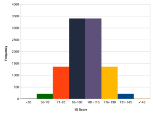
Normal distribution

A data set that has a normal distribution will have the majority of scores on or near the mean average. A normal distribution is also symmetrical: There are an equal number of scores above the mean as below it. In a normal distribution, scores become rarer and rarer the more they deviate from the mean.

An example of a normal distribution is IQ scores. As you can see from the histogram below, there are as many IQ scores below the mean as there are above the mean:

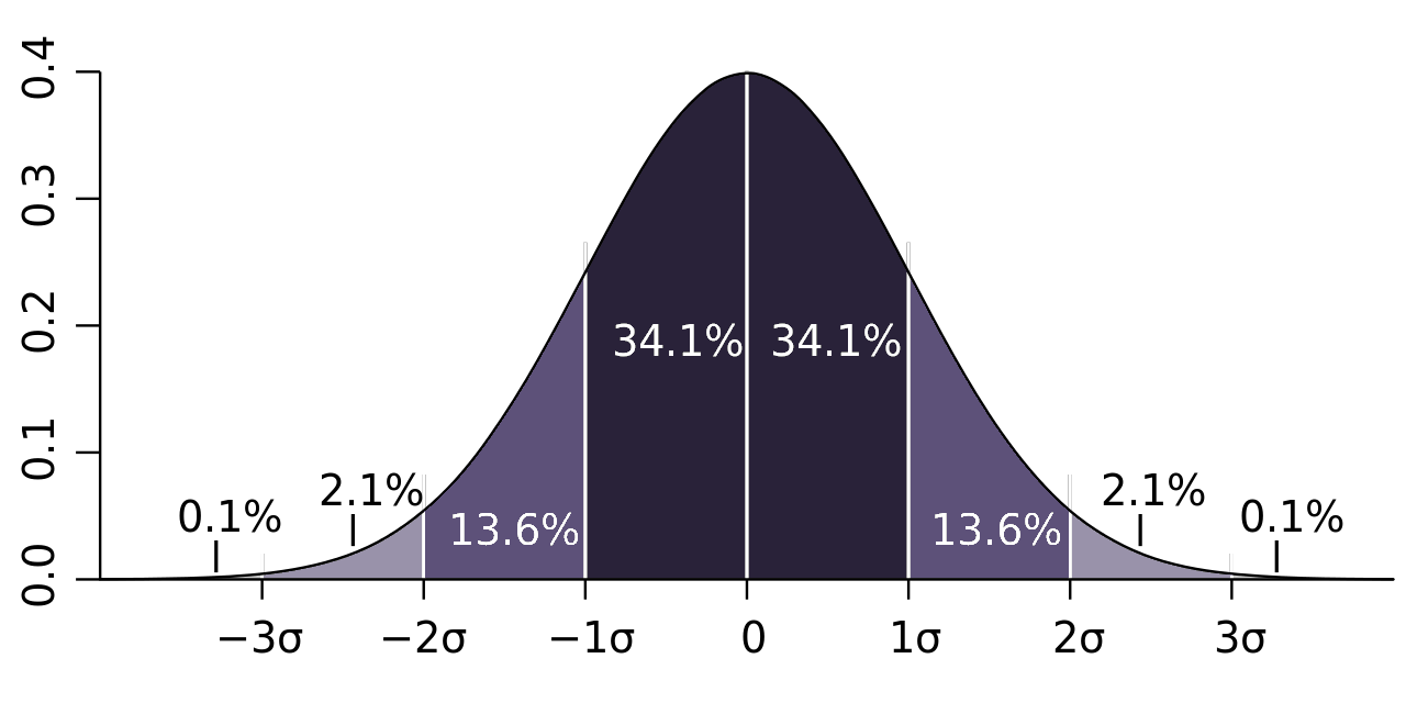
When plotted on a histogram, data that follows a normal distribution will form a bell-shaped curve like the one above.

Skewed distribution

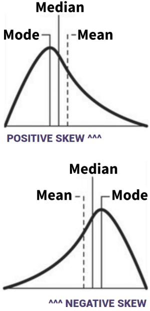A data set that has a skewed distribution will not be symmetrical: Scores are not distributed evenly either side of the mean.

Skewed distributions are caused by outliers: Freak scores that throw off the mean. Skewed distributions can be positive or negative:

• Positively skewed: A freakishly high score (or a cluster of low scores) makes the mean much higher than most of the scores, so most scores are below the mean.
  • Mean > Median > Mode
• Negatively skewed: A freakishly low score (or a cluster of high scores) makes the mean much lower than most of the scores, so most scores are above the mean.
  • Mean < Median < Mode

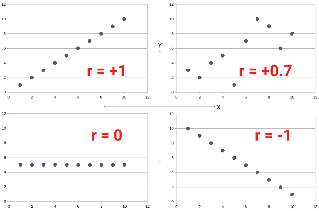
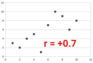
Correlation

Correlation refers to how closely related two (or more) things are related. For example, hot weather and ice cream sales may be positively correlated: When hot weather goes up, so do ice cream sales.

Correlations are measured mathematically using correlation coefficients (r). A correlation coefficient will be anywhere between +1 and -1:

• r=+1 means two things are perfectly positively correlated: When one goes up, so does the other by the same amount
• r=-1 means two things perfectly negatively correlated: When one goes up, the other goes down by the same amount
• r=0 means two things are not correlated at all: A change in one is totally independent of a change in the other

The following scattergrams illustrate various correlation coefficients:

Presentation of data

Tables

Tables are ways of presenting data. They can present raw data (data tables) or summarise results (results tables).

For example, the behavioural categories table above presents the raw data of each student in this made-up study. But in the results section, researchers might include another table that compares average anxiety rating scores for males and females.

Scattergrams

A scattergram illustrates two variables for various data points.

For example, each dot on the correlation scattergram opposite could represent a student. The x-axis could represent the number of hours the student studied, and the y-axis could represent the student’s test score.

Bar charts

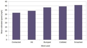A bar chart illustrates discrete data categories for comparison. The x-axis lists the categories and the y-axis illustrates the different results between the categories.

For example, the results of Loftus and Palmer’s study into the effects of different leading questions on memory could be presented using the bar chart above. It’s not like there are categories in-between ‘contacted’ and ‘hit’, so the bars have gaps between them (unlike a histogram).

Histograms

A histogram is a bit like a bar chart but is used to illustrate continuous or interval data (rather than discrete data or whole numbers).

For example, it’s not like you can only weigh 100kg or 101kg – there are many intervals in between. The x axis on the histogram opposite organises this continuous data (i.e. the in-between scores) into categories. The y axis illustrates the frequency of scores within each category.

Because the data on the x axis is continuous, there are no gaps between the bars.

Line graph

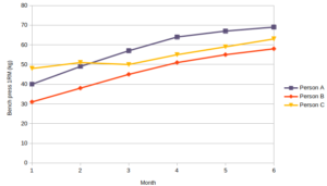Like a histogram, a line graph (sometimes called a frequency polygon) also illustrates continuous data. But whereas a histogram can only represent one data category, a line graph can illustrate multiple data categories.

For example, the line graph above illustrates 3 different people’s progression in a strength training program over time.

Pie chart

Pie charts illustrate how commonly different things occur relative to each other. In other words, they provide a visual representation of percentages.

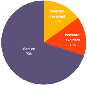
For example, the frequency with which different attachment styles occurred in Ainsworth’s strange situation could be represented by the pie chart opposite.

Inferential testing

Probability and significance

The point of inferential testing is to see whether a study’s results are statistically significant, i.e. whether any observed effects are as a result of whatever is being studied rather than just random chance.

For example, let’s say you are studying whether flipping a coin outdoors increases the likelihood of getting heads. You flip the coin 100 times and get 52 heads and 48 tails. Assuming a baseline expectation of 50:50, you might take these results to mean that flipping the coin outdoors does increase the likelihood of getting heads. However, from 100 coin flips, a ratio of 52:48 between heads and tails is not very significant and could have occurred due to luck. So, the probability that this difference in heads and tails is because you flipped the coin outside (rather than just luck) is low.

Probability is denoted by the symbol p. The lower the p value, the more statistically significant your results are. You can never get a p value of 0, though, so researchers will set a threshold at which point the results are considered statistically significant enough to reject the null hypothesis. In psychology, this threshold is usually <0.05, which means there is a less than 5% chance the observed effect is due to luck and a >95% chance it is a real effect.

Type 1 and type 2 errors

When interpreting statistical significance, there are two types of errors:

• Type 1 error (false positive): When researchers conclude an effect is real (i.e. they reject the null hypothesis), but it’s actually not
  • E.g. The p threshold is <0.05, but the researchers’ results are among the 5% of fluke outcomes that look significant but are just due to luck
• Type 2 error (false negative): When researchers conclude there is no effect (i.e. they accept the null hypothesis), but there actually is a real effect
  • E.g. The p threshold is set too low (e.g. <0.01), and the data falls short (e.g. p=<0.02)

Increasing the sample size reduces the likelihood of type 1 and type 2 errors.

---

Key maths skills made easy!

The research methods section of the colourful and concise revision guide includes simple explanations and worked examples of all the key mathematical and statistical skills needed for exam success, including: Which statistical test to use, how to use critical values tables, the sign test, and standard deviation.

---

Types of statistical test

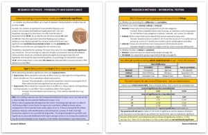
Note: The inferential tests below are needed for A level only, if you are taking the AS exam, you only need to know the sign test.

There are several different types of inferential test in addition to the sign test. Which inferential test is best for a study will depend on the following three criteria:

• Whether you are looking for a difference or a correlation
• Whether the data is nominal, ordinal, or interval
  • Nominal: Tallies of discrete categories
    • E.g. at the competition there were 8 runners, 12 swimmers, and 6 long jumpers (it’s not like there are in-between measurements between ‘swimmer’ and ‘runner’)
  • Ordinal: Whole numbers that can be ordered, but are not necessarily precise measurements
    • E.g. First, second, and third place in a race
    • E.g. Ranking your mood on a scale of 1-10
  • Interval: Standardised units of measurement (that can include a decimal point)
    • E.g. Weights in kg
    • E.g. Heights in cm
    • E.g. Times in seconds
• Whether the experimental design is related (i.e. repeated measures) or unrelated (i.e. independent groups)

The following table shows which inferential test is appropriate according to these criteria:

	Test of difference		Test of correlation
	Unrelated	Related
Nominal	Chi squared	Sign test	Chi squared
Ordinal	Mann Whitney	Wilcoxon	Spearman’s rho
Interval	Unrelated t test	Related t test	Pearson’s r

Note: You won’t have to work out all these tests from scratch, but you may need to:

• Say which of the statistical tests is appropriate (i.e. based on whether it’s a difference or correlation; whether the data is nominal, ordinal, or interval; and whether the data is related or unrelated).
• Identify the critical value from a critical values table and use this to say whether a result (which will be given to you in the exam) is statistically significant.

The sign test

The sign test is a way to calculate the statistical significance of differences between related pairs (e.g. before and after in a repeated measures experiment) of nominal data. If the observed value (s) is equal or less than the critical value (cv), the results are statistically significant.

Example: Let’s say we ran an experiment on 10 participants to see whether they prefer movie A or movie B.

Participant	Movie A rating	Movie B rating	Sign
A	3	6	B
B	3	3	n/a
C	5	6	B
D	4	6	B
E	2	3	B
F	3	7	B
G	5	3	A
H	7	8	B
I	2	6	B
J	8	5	A

• The most important thing in the sign test is not the actual amount (e.g. 4, 6, etc.), but the sign – i.e. whether they preferred movie A or movie B. You exclude any results that are the same between the pairs.
  • n = 9 (because even though there are 10 participants, one participant had no change so we exclude them from our calculation)
  • B = 7
  • A = 2
• Look to see if your experimental hypothesis is two-tailed (i.e. a change is expected in either direction) or one-tailed (i.e. change is expected to go in one direction)
  • In this case our experimental hypothesis is two-tailed: Participants may prefer movie A or movie B
  • (The null hypothesis is that participants like both movies equally)
• Find out the p value for the example (this will be provided in the exam)
  • In this case, let’s say it’s 0.1
• Using the information above, look up your critical value (cv) in a critical values table (this will be provided in the exam)
  • n = 9
  • p = 0.1
  • The experimental hypothesis is two-tailed
  • So, in this example, our critical value (cv) is 1
• Work out the observed value (s) by counting the number of instances of the less frequently occurring sign (A in this case)
  • In this example, there are 2 As, so our observed value (s) is 2
• In this example, the observed value (2) is greater than the critical value (1) and so the results are not statistically significant. This means we must accept the null hypothesis and reject the experimental hypothesis.

---

<<<Biopsychology